Sensorimotor behavior in a changing environment

An E. coli cell can't learn how its chemical surroundings change without swimming through them, so what it senses depends on how it has swum, and where it swims depends on what it has sensed. It's a loop with no obvious place to start. Celani and Vergassola (2010) put the same thing from the cell's side: sensing and motility are entangled, because the bacterium "must run to measure variations in the concentrations." This page follows that loop and asks two questions about it. Why does the cell's response have the shape it has, and what happens to the best strategy when swimming gets more costly or the water starts to move?

The loop, in numbers

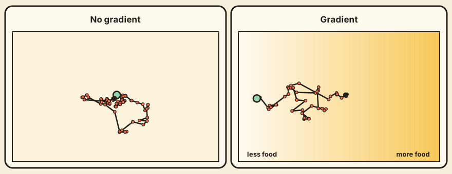
With no attractant around, E. coli swims at about 20 micrometres per second in runs whose lengths are random, with a mean near one second, and tumbles for about a tenth of a second. Each tumble turns the cell to a new heading, and after a few runs and tumbles its path is hard to tell from a random walk. observed Celani and Vergassola take these values from earlier measurements. When attractant is present, the chemotactic pathway changes how long runs last, and that's the whole steering system. No rudder, just a stopwatch.

They write the rate of switching from running to tumbling as a baseline rate times one minus a weighted sum of the concentrations the cell has recently detected. The weights are a response function K, which they take from a tethered-cell experiment: after a short pulse of aspartate, the bias of the flagellar motor rises and then undershoots, and the two lobes have nearly equal areas. observed The curve is an average over several cells. Equal lobes mean that a steady background adds nothing to the sum, so only recent change moves the tumbling rate. We read this as the behavioral side of the adaptation in C5. inferred

Why the response has this shape, when climbing wants another

The shape poses a puzzle. An earlier explanation says that equal lobes filter out the constant background so the cell can sense gradients whatever the level. Fair enough. But Celani and Vergassola point out that climbing a known gradient is done best by a single positive lobe, as de Gennes had noted, because a negative lobe cuts the drift up the gradient. Sensing and climbing ask for different responses, and the cell can only have one.

Their move was to ask what a cell should do when it can't know which gradient it will meet. For each possible response and run time they computed how much attractant the cell intercepts, which they call uptake, in any concentration profile. For each response they found the worst profile, and then picked the response whose worst case is best. This is called a maximin strategy, and it's the strategy of a cautious gambler who plans for the house to cheat. modeled The best response has a zero integral, as measured cells do. Using the rotational diffusion of an ellipsoid with axes of 1 and 0.25 micrometres in water, their predicted curve lies close to the measured one. modeled In their linear theory, it's also the only response that never does worse than a swimmer with the same runs and no chemotaxis.

They then simulated a population in a chemostat, a vessel with a steady slow inflow of nutrient, in which each cell's uptake fluctuates. Cells with a zero-integral response had smaller fluctuations in uptake, and because growth rate rises with uptake at a slowing pace, those cells excluded the others. modeled

The evidence has limits. The match is to one measured curve averaged over several cells. The theory assumes weak signals and scores a response by uptake, and the authors note that some attractants are only signposts that cells don't eat. We don't know whether a different performance measure would give the same curve.

A cost that moves the optimum

Taylor and Stocker (2012) moved the setting from a gut-like colony to open water. They ran direct numerical simulations of a patch of dissolved nutrient released into turbulent seawater, with motile and nonmotile bacteria competing for it. Motile cells swim up the gradient at a chemotactic velocity that rises with the gradient up to a maximum. modeled

Turbulence stirs the patch into thin filaments, and motile cells gather in them. With a maximum chemotactic velocity of 20 micrometres per second and strong turbulence, the motile cells took up 23 percent more nutrient than the nonmotile ones 13.2 seconds after release. The benefit nearly vanished after 50 seconds, although 59 percent of the nutrient was still there, because it had been mixed to uniformity. modeled The feast was still on the table. It just wasn't anywhere in particular.

Swimming costs energy. In the model, the benefit rises about linearly with chemotactic velocity while propulsive power rises as the square of swimming speed, so an optimum appears. In intermediate turbulence it fell at 15 to 25 micrometres per second, matching speeds recorded for several marine bacteria. modeled For E. coli, whose maximum chemotactic velocity they cite as 0.6 to 13.8 micrometres per second, the model gave at most a 15 percent gain at 5 micrometres per second. Weaker turbulence favored chemotaxis for small patches, and in strong turbulence the benefit was fivefold smaller. Low nutrient input favored nonmotile cells, which fits the abundance of nonmotile clades in the open ocean. inferred

The authors say that ocean observations of motility are too few to test these predictions, and that extra costs, such as building flagella, could lower the optimum further.

What neither paper reaches

Neither paper predicts a full distribution of paths. Celani and Vergassola derive diffusion and drift for the population, and Taylor and Stocker give uptake. Neither treats two cues that disagree, so we can't say here what a cell does when an attractant and a repellent conflict.

What does a cell do when one cue says go and another says stop?

We don't know, from these papers at least. C6 asked how well a pathway tells inputs apart. These papers ask what a swimming cell does with the signal once it has it.

What you should be able to do after reading

Predict which way the drift and spread of swimming cells shift under a new gradient or a changed swimming cost, and say why.

A quick test: first, give a cell the zero-integral response and place it in a steady, uniform background. Say what happens to its tumbling rate and to its path. Then raise the cost of swimming in the Taylor and Stocker model, and say which way the best chemotactic velocity moves and why.

References

- Celani, A., & Vergassola, M. (2010). Bacterial strategies for chemotaxis response. Proceedings of the National Academy of Sciences, 107(4), 1391-1396. doi:10.1073/pnas.0909673107
- Taylor, J. R., & Stocker, R. (2012). Trade-offs of chemotactic foraging in turbulent water. Science, 338(6107), 675-679. doi:10.1126/science.1219417